Gaussian Mixture for dimensionality reduction

Features : 28 numerical features (from PCA by the dataset owner) + transaction amount of credit card transactions (284,807 samples)

Label : 0/1 (non-fraud/fraud transaction)

Number of Samples : 284,807

Dataset Link : www.kaggle.com/mlg-ulb/creditcardfraud

In this project, I worked with a credit card transactions dataset containing 28 "uninterpretable" numerical features of each transaction (the source says they are from principal components analysis) plus a transaction amount, along with a binary fraud (1)/non-fraud (0) label.

The dataset is unbalanced, meaning that one class has much, much more samples than the other. Here, we have 99.83% non-fraud transactions and 0.17% fraud transactions. This is quite likely in reality, as fraudulent credit card transactions should happen only a small amount of times compared to normal, healthy transactions. Thus, detecting fraudulent transactions is an outlier detection problem.

Data Analysis Steps :

1. Fitted a uni-variate Gaussian distribution on each SINGLE feature in an UNSUPERVISED way, by fitting ALL samples (fraud + non-fraud).

2. Computed AUC (Area under the ROC Curve) with prediction scores (=how likely it is for a sample to belong to the distribution) for each single-feature model from step 1.

3. Made 3 different subsets of data, with features that have AUC larger than 0.9, 0.88, and 0.85 (each with 5, 7, and 9 features)

4. Plotted the distributions of each of the three subsets :

• Features with AUC > 0.9 (5 features out of 29)

This is the supervised plot of the first subset, with only 5 most informative features with AUC > 0.9. There is an apparent contrast between the distributions of the FRAUD (short and wide) and the NON-FRAUD (tall and narrow) distributions. In high level, it looks like there are about 2 to 3 different Gaussians for FRAUD cases and about 1 to 2 different Gaussians for NON-FRAUD cases. that have greater variance than NON-FRAUD cases. It's also important to note that FRAUD data distribution is wider, meaning that it has greater variance. This confirms our assumption that the small amount of FRAUD transactions (0.17% of data) are OUTLIERS, which perform a greater variety of "non-conventional" behaviours.

• Features with AUC > 0.88 (7 features out of 29)

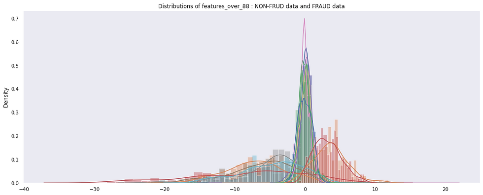
Now, it looks like there are more distinct Gaussians for FRAUD cases. There is still a contrast between the distributions of the FRAUD (shorter and wider) and the NON-FRAUD (tall and narrow) distributions, although not as distinctive than the previous subset. There are about 3 to 4 different Gaussians for FRAUD cases and about 1 to 3 different Gaussians for NON-FRAUD cases.

• Features with AUC > 0.85 (9 features out of 29)

Now, it looks like there are about 4 to 5 Gaussians for FRAUD data. But this plot looks a bit more clogged and confusing than the plots of the two previous subsets.

Further Steps :

1. Using the three subsets of data, I fitted two multi-variate Gaussian distributions on each subset in a SUPERVISED way, by fitting one Gaussian distriution (G1) on NON-FRAUD transactions only and the other (G2) on FRAUD transactions only.

2. Used a strategy where if a transaction's probability of being generated by G1 is less than a constant times the probability of being generated by G2, then transaction is fraudulent.

Result :

Gaussian Mixture Model that resulted in the highest training Recall (of 80.9%) was the one using :

• first subset of 5 features with AUC > 0.9

• FRAUD distribution with 3 Gaussians

• NON-FRAUD distribution with 2 Gaussians

This is amazingly close to what we already observed in the plots above!

Self-Reflection:

I learned that Gaussian Mixture Model is another effective dimensionality reduction tool (sort of, only to 2-D, though), by making it possible to plot the distribution of different classes and observe the differences.

My Colab Notebook of this project can be found at :

github.com/lukysummer/Fraud-Detection-using-Gaussian-Mixtures/blob/main/Creditcard_Fraud_Detection.ipynb